Carlo Debernardi

So as of late I have been chatting with a colleague – a labor economist – about work-related or occupational injuries. A lingering problem in this area is that (at least in Italy) the phenomenon of under reporting of on-the-job injuries is incredibly widespread. Which of course makes the phenomenon as a whole hard to tackle because we cannot really take administrative data on face value nor make the usual assumptions of random measurement errors and the like.

Now, during the same days I was also reading Jaynes’ Probability Theory: The Logic of Science, because I love old books and grumpy old authors with their hot takes and stinging remarks. From paragraph 6.10 onwards Jaynes introduces a compound estimation problem. He lays out three versions of the problem and then keeps the one with an analogy from physics in the subsequent discussion, here I report the example which is the most intuitive to me:

In the general population, there is a frequency p at which any given person will contract a certain disease within the next year; and then another frequency θ that anyone with the disease will die of it within a year. From the observed variations {c1, c2, . . .} of deaths from the disease in successive years (which is a matter of public record), estimate how the incidence of the disease {n1, n2, . . .} is changing in the general population (which is not a matter of public record).

Now. Do you see it?

Jaynes is modeling a two step procedure where the first step is producing a count of some stuff according to a Poisson distribution, but instead of observing the true count we only get information on a subset of it with a certain probability.

Ta daaa. This ringed a bell for me as I though of the true number of on-the-job injuries as our true count, and under reporting is essentially 1 − θ, i.e. the complement of the probability of actually observing an injury. Jaynes then shows that this compounded process is equivalent to a Poisson likelihood with the rate multiplied by θ.

Reading around online I found out a little more about this: Poisson distributions can be broken down into independent categorical “pieces” by just multiplying their rate by a fraction, the result is still a Poisson distribution and the total expectation is the same, it’s called poisson thinning.

So of course my next step was jumping right into modeling…

Fetch me some data!

Administrative data are not always easy to access, they are often messy or extremely aggregated. To my surprise, I found out that INAIL¹ data of on-the-job injuries are quite well maintained and documented. I downloaded the data for Piedmont (my home region) in the time span 2015-2024.

That’s good, but it would be nice to have an idea of how many workers were in each sector over time, to get a sense of how likely it is for a person to be injured while working. Unfortunately the only public source I could find is an INPS dashboard² which – for some reason – refuses to provide unaggregated data to a reasonable level if even just one of the categories requested is not numerous enough (I’m surely gonna breach someone’s privacy by knowing how many coal miners are there³!).

Anyway, in order not to go crazy I restrained myself to the manufacturing sector, which arguably might be among the ones with a high incidence of injuries, and is composed of 24 sub-sectors, so we can expect a reasonable heterogeneity.

Now, this is a blogpost about Poisson thinning and a cool model, not a labor economics dissertation, which means I’m going to gloss over a ton of details. I’ll ignore the difference between male and female workers, blue and white collars, full-time and part-time contracts, hiring and firing, administrative distinctions between different kinds of on-the-job injuries, etc.

So, for this very basic exercise I will be looking only at sub-sectors and injury severity. This last one I aggregated into 8 categories ranging from “just rest at home for some days” to death⁴. I will also consider the process fixed over time for two reasons: I only have one yearly observation per subsector and in the aggregate both the number of workers and the number of reported injuries looks very stable.

To the model! Version 1

Actually, let’s get Version 0 out of the way first. The naivest thing we could do is just model the count of injuries by sector as a Poisson distribution with a global intercept and a sector specific rate, adding in the log of the number of workers so that the rate is measured per capita. Of course we will be working on the log scale, for numerical stability; after all, injuries are hopefully a relatively rare event, which mean working with small probabilities.

This is our baseline Poisson regression:

I_s, y ∼ LogPoisson(α+ln(w_s, y)+h_s)

Where s is an index over sectors, y is an index over years, I is the count of injuries injuries and h is the “hazard” of each subsector.

Now, this would be our vanilla Poisson regression, but we are here for thinning. So let’s move on to Version 1.

Version 1, for real

We will break down our starting model into 8 components, indexed by k, so that we will be able to distinguish between different levels of severity:

I_s, k, y ∼ LogPoisson(α+ln(w_s, y)+h_s+S_k)

Duh, you just added one term.

Yes, since we are working on the log scale, multiplication turns into addition. But I haven’t revealed the cool part yet. S is meant to be a vector of 8 values partitioning the rest of the likelihood but preserving the total, which means it has to sum to 1 in the natural scale. How can we do this?

S_k = LogSoftmax(η_k)

η₀ = 0

That’s it!

If you have ever used a multinomial logistic regression in your life, or messed with neural networks, you know what I’m talking about. If you haven’t, think of softmax as a function which enables you to normalize a vector to sum to one. We could just divide the elements by the total, but if those elements are parameters then we would have to work with an awkward geometry in case we want, for example, to introduce predictors for those parameters. The only slightly unusual thing is doing softmax on the log scale, but luckily Stan has us covered with a dedicated implementation.

We are also fixing the first element of the vector for identifiability, otherwise multiple parameters configuration could result in the same outcome. This means we are using the least severe injury conditions as a reference category.

Since we are going to fit this model in Stan we will also need priors.

α ∼ N(−4,1)

This should result in an average individual rate of yearly injuries of about 2%, and most of the probability mass (i.e. taking 3 sds above the mean) should be below 36%. That is hell of a wide prior in this case, if we had a single sector with an injury rate that high it would be on all headlines, if the overall average rate was this high, well… Anyway.

Given that this is just a blogpost and the model is small I will not put in the work of figuring out decent priors for η. Stan will probably figure it out in this case, but don’t do this at home. I’m just hoping it will not explode.

Since we are here though we can as well put some partial pooling on our subsector intercepts because why not, it’s hard to go wrong with pooling information:

h ∼ N(0,σ_h)

σ_h ∼ Exponential(1)

Notice that this implies weak identifiability. It should not be an issue in this case, but if we wanted we could address it by taking one sector as reference category (meh) or constrain the h values to be a sum-to-zero vector (I personally like it better).

Ok, we are done. The full Stan implementation of the model is here. Let’s see if it works.

The model runs smoothly, no warnings, no divergences; Rhat, ESS and trace plots look ok. Let’s take a look at the results.

Our guess for the global intercept was reasonable, it’s estimated as -4.2 (-4.5, -3.9). What about the subsectors?

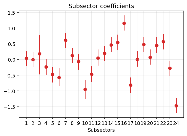
Here they are. Quite a lot of heterogeneity! Other notable, and in retrospect reasonable, things are:

• Subsector 3 has a LOT of uncertainty. This is due to the fact that there are actually very few workers there (it’s the tobacco industry, <100 workers) and almost no injuries. Partial pooling is doing it’s job here.
• Subsector 16 (metalworking) is the one with the highest rate of reported injuries.
• Subsector 24 (repair and maintenance of industrial machines) is the one with the lowest.

What about the severity composition? Here the estimates of our poisson thinning probabilities once we bring them back to their natural 0-1 scale (notice the log on the y axis though).

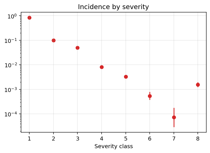
Unsurprisingly the rate of injuries declines with their severity. The only exception to this monotonic trend is level 8. Taken at face value, this would suggests that – conditional on getting injured – death is a more likely outcome than survival with very high levels of physical impairment. If this were true, it could be linked to biological properties of human bodies, but alternative explanations are possible (e.g. we are taking the severity classes at face value, but these are assigned based on expert judgement). The reality is likely a mix of things.

On a less speculative ground, we can notice how the uncertainty bounds around our point estimates basically disappear, except for the severity classes 6 and 7, which are indeed very rare in the dataset.

Finally, we could assess how our model fits to the data. Let’s start, for example, by looking at Subsector 16. The grey boxplots are our model predictions, red lines mark true values, and we are pooling all the years.

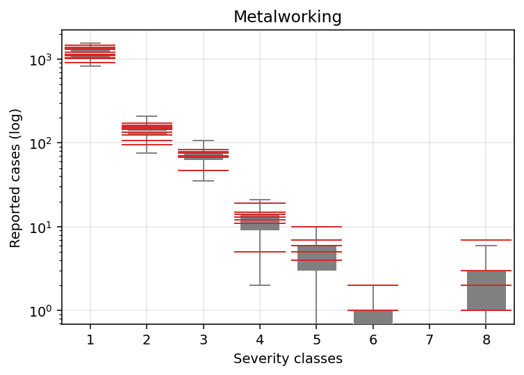
I would say pretty good for a first iteration.

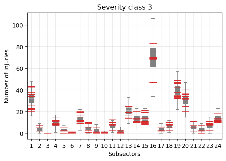
Now, let’s look at it from another angle and compare, say, severity class 3 across sectors.

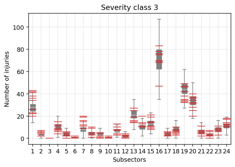
Again, I would say pretty good for a first iteration. But we also start to see that our model does not perform equally for all subsectors. For example, injury rate reports in Subsector 7 (woodworking) look systematically underestimated. Our estimates for Subsector 19 (coke and oil refinement) instead seem skewed towards the higher end. I’m unsure of what is happening with Subsector 1 (food processing), but there seems to be more variation in the data than predicted by the model.

All of this is likely the consequence of the fact that this version of our model fixes a single severity distribution globally which is uniformly applied to all subsectors. Even intuitively we would expect such a strong assumption not to hold.

So, time for a little more heterogeneity…

To the model! Version 2

Now, a very simple thing to do would be to simply allow every subsector to fit it’s own distribution like a glove, by giving them completely independent coefficients. This is the maximum degree of heterogeneity possible, but we are bayesian in this house, so we are trying to squeeze every little bit of information out of our data. We do not believe in completely independent things.

Another alternative would be to regularize our estimates in a similar way to what we have done with our h values for the subsectors. But that would be more of the same…

Let’s take a step back and take a look at our h values, the subsector hazards. Well, it would be reasonable to expect that subsector with higher hazard – for example, in which highly dangerous tasks are widespread – will not only display higher injury counts, but shifts in the severity distribution. We are already estimating the h values for each subsector, we just have to find a way to make the severity of the injury – and not only their number – to depend upon them.

With a little bit of foreshadowing we have parametrized the incidence of the severity classes as a softmax, so that we could introduce predictors in their definition. And that is what we are going to do! We are simply replacing our old softmax with a new one:

S_k = LogSoftmax(η_k+γ_kh_s)

What exactly are we doing? Well, the h values are the same we saw earlier. The new gamma values (one for each severity class) represent shifts in the severity distribution associated with variations in h. We will give them a standard normal prior.

The Stan implementation of this version of the model is available here.

This version of the model takes a little longer to run, but again samples fine. The estimate for the global intercept is unchanged. Let’s take a look at the h values and compare them with the previous ones.

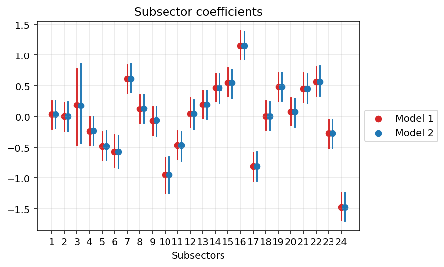
Yep, as I was hoping this has not impacted the estimates of our h values. But they now have the power to affect the severity distributions through the gammas… Speaking of which:

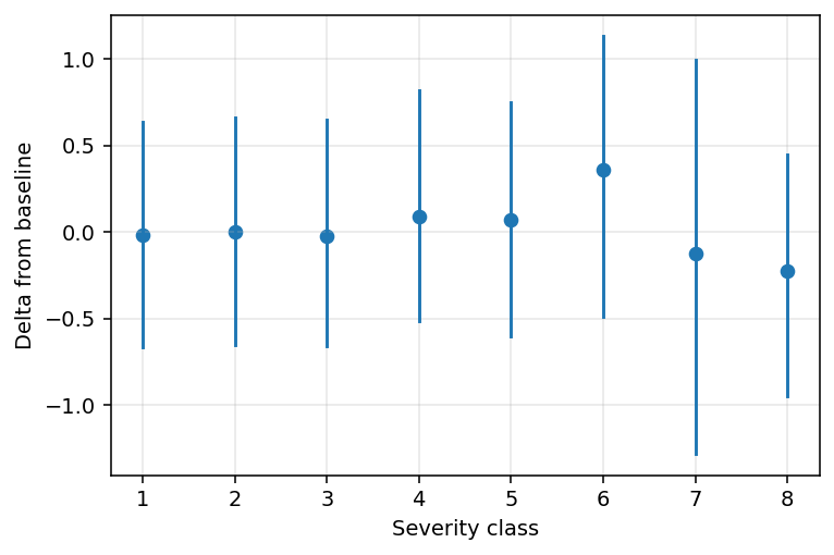
Welp. Seems like we cannot really say anything about shifts in the severity distribution…

In any case I think this is a pretty cool version of the model, with a single latent quantity determining both the number and the severity of injuries. But fine, I will surrender and go on to a more flexible Version 3.

Version 3. Not over yet?

Here we are with the final (for now) version of the model, in which instead of imposing parametric restrictions on the shape of the severity distribution, we let it vary by sector. Of course, again, we are partially pooling because we are in bayes land.

S_k = LogSoftmax(η_k+ζ_ks)

ζ_k ∼ N(0,ψ_k)

ψ_k ∼ Exponential(1)

This is a little Greek galore, but the underlying idea is the same as the partial pooling we used for the h values. The idea is that, for each severity class, we allow sectors to have different incidences, but they all share a grand mean.

Since we are here, we will also define decent priors over the η values.

η_k ∼ N(−k,1)

Again, the Stan implementation is here.

The model runs kind of ok, but ESS and Rhat start complaining a little. To fix those I should probably address the weak identification of the h values. But we are here for the juice, let’s take a look at the severity rates for a selected group of subsectors:

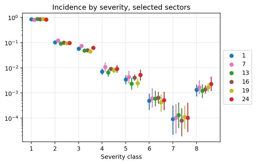
There is, indeed, heterogeneity. The scale of it is just so tiny because we are working with very small quantities.

Let’s see if this improved our predictions by again looking at Severity class 3:

The weird cases of before look much crisper to me!

But, what about under reporting?

Yes. I admit. The opening was a trap. We could indeed model under reporting and make inferences about the true rate of injuries, and poisson thinning would be a good tool to address the issue. Just add one term to the product (or sum, depending on if you look at it on the log scale) and give a parametrization to it.

The point is, doing that would require much finer data about dimensions we know affect the probability of reporting injuries – like for example firm size, or the presence of unions – and a review of the available evidence on the plausible scale of these effects. Even evidence from surveys of workers could be useful to inform such an attempt.

But I do not have access to such information right now, and this blog post is already way too long. Anyway, by writing this I got to understand a little more count models, and I think being able to sort of separately but still jointly model the rate and the shape of a phenomenon is nice.